Continuous Queries on Dynamic Tables

Analyzing Data Streams with SQL #

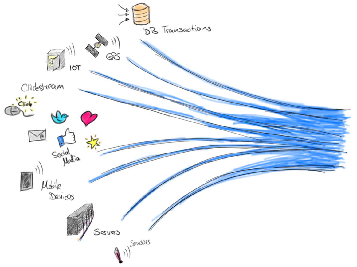
More and more companies are adopting stream processing and are migrating existing batch applications to streaming or implementing streaming solutions for new use cases. Many of those applications focus on analyzing streaming data. The data streams that are analyzed come from a wide variety of sources such as database transactions, clicks, sensor measurements, or IoT devices.

Apache Flink is very well suited to power streaming analytics applications because it provides support for event-time semantics, stateful exactly-once processing, and achieves high throughput and low latency at the same time. Due to these features, Flink is able to compute exact and deterministic results from high-volume input streams in near real-time while providing exactly-once semantics in case of failures.

Flink’s core API for stream processing, the DataStream API, is very expressive and provides primitives for many common operations. Among other features, it offers highly customizable windowing logic, different state primitives with varying performance characteristics, hooks to register and react on timers, and tooling for efficient asynchronous requests to external systems. On the other hand, many stream analytics applications follow similar patterns and do not require the level of expressiveness as provided by the DataStream API. They could be expressed in a more natural and concise way using a domain specific language. As we all know, SQL is the de-facto standard for data analytics. For streaming analytics, SQL would enable a larger pool of people to specify applications on data streams in less time. However, no open source stream processor offers decent SQL support yet.

Why is SQL on Streams a Big Deal? #

SQL is the most widely used language for data analytics for many good reasons:

• SQL is declarative: You specify what you want but not how to compute it.
• SQL can be effectively optimized: An optimizer figures out an efficient plan to compute your result.
• SQL can be efficiently evaluated: The processing engine knows exactly what to compute and how to do so efficiently.
• And finally, everybody knows and many tools speak SQL.

So being able to process and analyze data streams with SQL makes stream processing technology available to many more users. Moreover, it significantly reduces the time and effort to define efficient stream analytics applications due to the SQL’s declarative nature and potential to be automatically optimized.

However, SQL (and the relational data model and algebra) were not designed with streaming data in mind. Relations are (multi-)sets and not infinite sequences of tuples. When executing a SQL query, conventional database systems and query engines read and process a data set, which is completely available, and produce a fixed sized result. In contrast, data streams continuously provide new records such that data arrives over time. Hence, streaming queries have to continuously process the arriving data and never “complete”.

That being said, processing streams with SQL is not impossible. Some relational database systems feature eager maintenance of materialized views, which is similar to evaluating SQL queries on streams of data. A materialized view is defined as a SQL query just like a regular (virtual) view. However, the result of the query is actually stored (or materialized) in memory or on disk such that the view does not need to be computed on-the-fly when it is queried. In order to prevent that a materialized view becomes stale, the database system needs to update the view whenever its base relations (the tables referenced in its definition query) are modified. If we consider the changes on the view’s base relations as a stream of modifications (or as a changelog stream) it becomes obvious that materialized view maintenance and SQL on streams are somehow related.

Flink’s Relational APIs: Table API and SQL #

Since version 1.1.0 (released in August 2016), Flink features two semantically equivalent relational APIs, the language-embedded Table API (for Java and Scala) and standard SQL. Both APIs are designed as unified APIs for online streaming and historic batch data. This means that,

a query produces exactly the same result regardless whether its input is static batch data or streaming data.

Unified APIs for stream and batch processing are important for several reasons. First of all, users only need to learn a single API to process static and streaming data. Moreover, the same query can be used to analyze batch and streaming data, which allows to jointly analyze historic and live data in the same query. At the current state we haven’t achieved complete unification of batch and streaming semantics yet, but the community is making very good progress towards this goal.

The following code snippet shows two equivalent Table API and SQL queries that compute a simple windowed aggregate on a stream of temperature sensor measurements. The syntax of the SQL query is based on Apache Calcite’s syntax for grouped window functions and will be supported in version 1.3.0 of Flink.

val env = StreamExecutionEnvironment.getExecutionEnvironment
env.setStreamTimeCharacteristic(TimeCharacteristic.EventTime)

val tEnv = TableEnvironment.getTableEnvironment(env)

// define a table source to read sensor data (sensorId, time, room, temp)
val sensorTable = ??? // can be a CSV file, Kafka topic, database, or ...
// register the table source
tEnv.registerTableSource("sensors", sensorTable)

// Table API
val tapiResult: Table = tEnv.scan("sensors")   // scan sensors table
 .window(Tumble over 1.hour on 'rowtime as 'w) // define 1-hour window
 .groupBy('w, 'room)                           // group by window and room
 .select('room, 'w.end, 'temp.avg as 'avgTemp) // compute average temperature

// SQL
val sqlResult: Table = tEnv.sql("""
 |SELECT room, TUMBLE_END(rowtime, INTERVAL '1' HOUR), AVG(temp) AS avgTemp
 |FROM sensors
 |GROUP BY TUMBLE(rowtime, INTERVAL '1' HOUR), room
 |""".stripMargin)

As you can see, both APIs are tightly integrated with each other and Flink’s primary DataStream and DataSet APIs. A Table can be generated from and converted to a DataSet or DataStream. Hence, it is easily possible to scan an external table source such as a database or Parquet file, do some preprocessing with a Table API query, convert the result into a DataSet and run a Gelly graph algorithm on it. The queries defined in the example above can also be used to process batch data by changing the execution environment.

Internally, both APIs are translated into the same logical representation, optimized by Apache Calcite, and compiled into DataStream or DataSet programs. In fact, the optimization and translation process does not know whether a query was defined using the Table API or SQL. If you are curious about the details of the optimization process, have a look at a blog post that we published last year. Since the Table API and SQL are equivalent in terms of semantics and only differ in syntax, we always refer to both APIs when we talk about SQL in this post.

In its current state (version 1.2.0), Flink’s relational APIs support a limited set of relational operators on data streams, including projections, filters, and windowed aggregates. All supported operators have in common that they never update result records which have been emitted. This is clearly not an issue for record-at-a-time operators such as projection and filter. However, it affects operators that collect and process multiple records as for instance windowed aggregates. Since emitted results cannot be updated, input records, which arrive after a result has been emitted, have to be discarded in Flink 1.2.0.

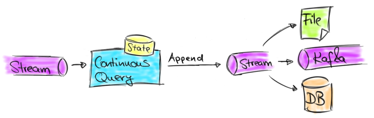
The limitations of the current version are acceptable for applications that emit data to storage systems such as Kafka topics, message queues, or files which only support append operations and no updates or deletes. Common use cases that follow this pattern are for example continuous ETL and stream archiving applications that persist streams to an archive or prepare data for further online (streaming) analysis or later offline analysis. Since it is not possible to update previously emitted results, these kinds of applications have to make sure that the emitted results are correct and will not need to be corrected in the future. The following figure illustrates such applications.

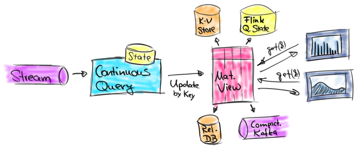
While queries that only support appends are useful for some kinds of applications and certain types of storage systems, there are many streaming analytics use cases that need to update results. This includes streaming applications that cannot discard late arriving records, need early results for (long-running) windowed aggregates, or require non-windowed aggregates. In each of these cases, previously emitted result records need to be updated. Result-updating queries often materialize their result to an external database or key-value store in order to make it accessible and queryable for external applications. Applications that implement this pattern are dashboards, reporting applications, or other applications, which require timely access to continuously updated results. The following figure illustrates these kind of applications.

Continuous Queries on Dynamic Tables #

Support for queries that update previously emitted results is the next big step for Flink’s relational APIs. This feature is so important because it vastly increases the scope of the APIs and the range of supported use cases. Moreover, many of the newly supported use cases can be challenging to implement using the DataStream API.

So when adding support for result-updating queries, we must of course preserve the unified semantics for stream and batch inputs. We achieve this by the concept of Dynamic Tables. A dynamic table is a table that is continuously updated and can be queried like a regular, static table. However, in contrast to a query on a batch table which terminates and returns a static table as result, a query on a dynamic table runs continuously and produces a table that is continuously updated depending on the modification on the input table. Hence, the resulting table is a dynamic table as well. This concept is very similar to materialized view maintenance as we discussed before.

Assuming we can run queries on dynamic tables which produce new dynamic tables, the next question is, How do streams and dynamic tables relate to each other? The answer is that streams can be converted into dynamic tables and dynamic tables can be converted into streams. The following figure shows the conceptual model of processing a relational query on a stream.

First, the stream is converted into a dynamic table. The dynamic table is queried with a continuous query, which produces a new dynamic table. Finally, the resulting table is converted back into a stream. It is important to note that this is only the logical model and does not imply how the query is actually executed. In fact, a continuous query is internally translated into a conventional DataStream program.

In the following, we describe the different steps of this model:

1. Defining a dynamic table on a stream,
2. Querying a dynamic table, and
3. Emitting a dynamic table.

Defining a Dynamic Table on a Stream #

The first step of evaluating a SQL query on a dynamic table is to define a dynamic table on a stream. This means we have to specify how the records of a stream modify the dynamic table. The stream must carry records with a schema that is mapped to the relational schema of the table. There are two modes to define a dynamic table on a stream: Append Mode and Update Mode.

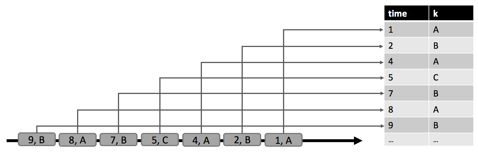
In append mode each stream record is an insert modification to the dynamic table. Hence, all records of a stream are appended to the dynamic table such that it is ever-growing and infinite in size. The following figure illustrates the append mode.

In update mode a stream record can represent an insert, update, or delete modification on the dynamic table (append mode is in fact a special case of update mode). When defining a dynamic table on a stream via update mode, we can specify a unique key attribute on the table. In that case, update and delete operations are performed with respect to the key attribute. The update mode is visualized in the following figure.

Querying a Dynamic Table #

Once we have defined a dynamic table, we can run a query on it. Since dynamic tables change over time, we have to define what it means to query a dynamic table. Let’s imagine we take a snapshot of a dynamic table at a specific point in time. This snapshot can be treated as a regular static batch table. We denote a snapshot of a dynamic table A at a point t as A[t]. The snapshot can be queried with any SQL query. The query produces a regular static table as result. We denote the result of a query q on a dynamic table A at time t as q(A[t]). If we repeatedly compute the result of a query on snapshots of a dynamic table for progressing points in time, we obtain many static result tables which are changing over time and effectively constitute a dynamic table. We define the semantics of a query on a dynamic table as follows.

A query q on a dynamic table A produces a dynamic table R, which is at each point in time t equivalent to the result of applying q on A[t], i.e., R[t] = q(A[t]). This definition implies that running the same query on q on a batch table and on a streaming table produces the same result. In the following, we show two examples to illustrate the semantics of queries on dynamic tables.

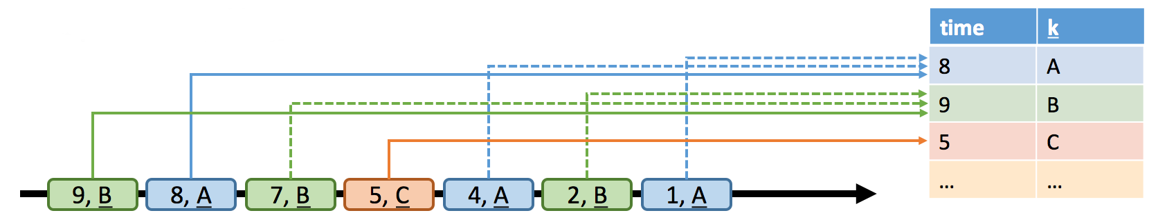
In the figure below, we see a dynamic input table A on the left side, which is defined in append mode. At time t = 8, A consists of six rows (colored in blue). At time t = 9 and t = 12, one row is appended to A (visualized in green and orange, respectively). We run a simple query on table A which is shown in the center of the figure. The query groups by attribute k and counts the records per group. On the right hand side we see the result of query q at time t = 8 (blue), t = 9 (green), and t = 12 (orange). At each point in time t, the result table is equivalent to a batch query on the dynamic table A at time t.

The query in this example is a simple grouped (but not windowed) aggregation query. Hence, the size of the result table depends on the number of distinct grouping keys of the input table. Moreover, it is worth noticing that the query continuously updates result rows that it had previously emitted instead of merely adding new rows.

The second example shows a similar query which differs in one important aspect. In addition to grouping on the key attribute k, the query also groups records into tumbling windows of five seconds, which means that it computes a count for each value of k every five seconds. Again, we use Calcite’s group window functions to specify this query. On the left side of the figure we see the input table A and how it changes over time in append mode. On the right we see the result table and how it evolves over time.

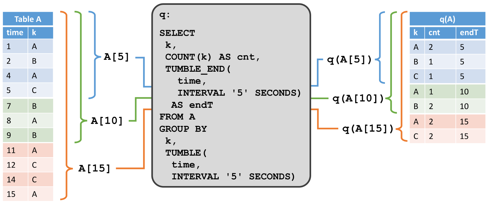
In contrast to the result of the first example, the resulting table grows relative to the time, i.e., every five seconds new result rows are computed (given that the input table received more records in the last five seconds). While the non-windowed query (mostly) updates rows of the result table, the windowed aggregation query only appends new rows to the result table.

Although this blog post focuses on the semantics of SQL queries on dynamic tables and not on how to efficiently process such a query, we’d like to point out that it is not possible to compute the complete result of a query from scratch whenever an input table is updated. Instead, the query is compiled into a streaming program which continuously updates its result based on the changes on its input. This implies that not all valid SQL queries are supported but only those that can be continuously, incrementally, and efficiently computed. We plan discuss details about the evaluation of SQL queries on dynamic tables in a follow up blog post.

Emitting a Dynamic Table #

Querying a dynamic table yields another dynamic table, which represents the query’s results. Depending on the query and its input tables, the result table is continuously modified by insert, update, and delete changes just like a regular database table. It might be a table with a single row, which is constantly updated, an insert-only table without update modifications, or anything in between.

Traditional database systems use logs to rebuild tables in case of failures and for replication. There are different logging techniques, such as UNDO, REDO, and UNDO/REDO logging. In a nutshell, UNDO logs record the previous value of a modified element to revert incomplete transactions, REDO logs record the new value of a modified element to redo lost changes of completed transactions, and UNDO/REDO logs record the old and the new value of a changed element to undo incomplete transactions and redo lost changes of completed transactions. Based on the principles of these logging techniques, a dynamic table can be converted into two types of changelog streams, a REDO Stream and a REDO+UNDO Stream.

A dynamic table is converted into a redo+undo stream by converting the modifications on the table into stream messages. An insert modification is emitted as an insert message with the new row, a delete modification is emitted as a delete message with the old row, and an update modification is emitted as a delete message with the old row and an insert message with the new row. This behavior is illustrated in the following figure.

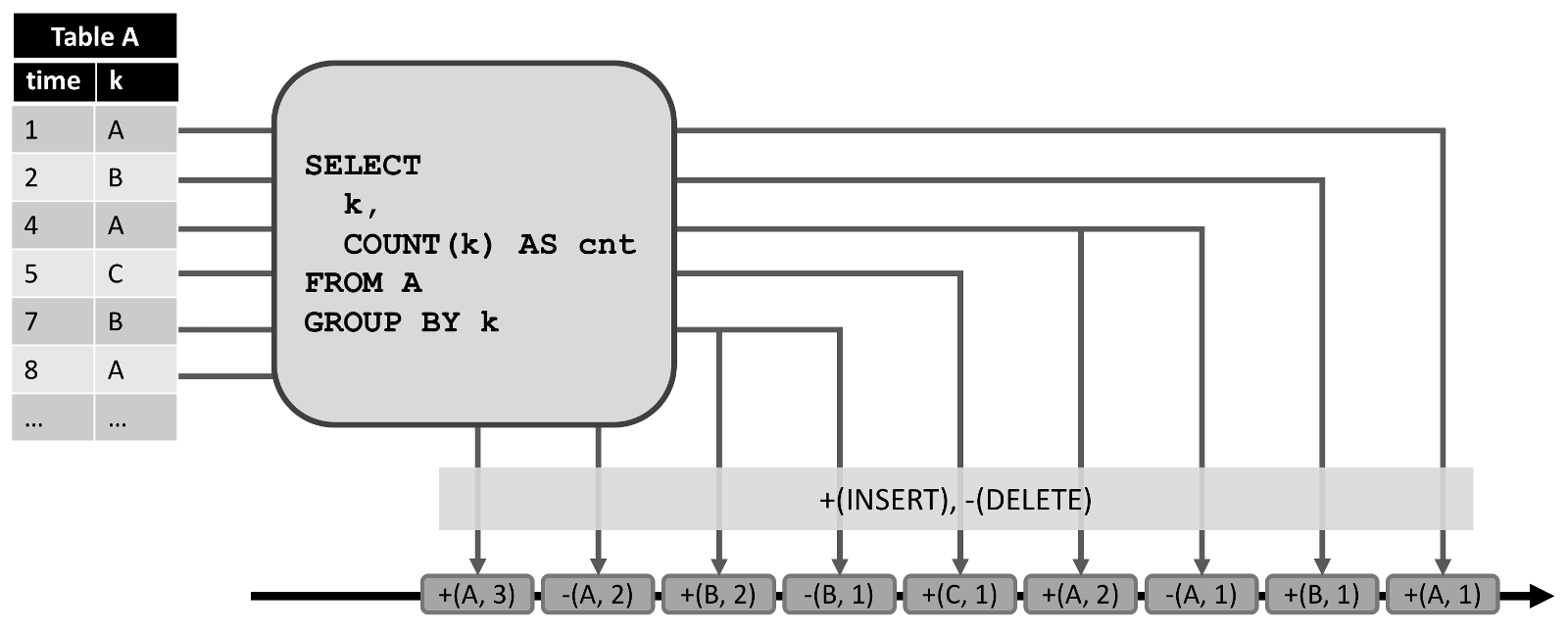
The left shows a dynamic table which is maintained in append mode and serves as input to the query in the center. The result of the query converted into a redo+undo stream which is shown at the bottom. The first record (1, A) of the input table results in a new record in the result table and hence in an insert message +(A, 1) to the stream. The second input record with k = ‘A’ (4, A) produces an update of the (A, 1) record in the result table and hence yields a delete message -(A, 1) and an insert message for +(A, 2). All downstream operators or data sinks need to be able to correctly handle both types of messages.

A dynamic table can be converted into a redo stream in two cases: either it is an append-only table (i.e., it only has insert modifications) or it has a unique key attribute. Each insert modification on the dynamic table results in an insert message with the new row to the redo stream. Due to the restriction of redo streams, only tables with unique keys can have update and delete modifications. If a key is removed from the keyed dynamic table, either because a row is deleted or because the key attribute of a row was modified, a delete message with the removed key is emitted to the redo stream. An update modification yields an update message with the updating, i.e., new row. Since delete and update modifications are defined with respect to the unique key, the downstream operators need to be able to access previous values by key. The figure below shows how the result table of the same query as above is converted into a redo stream.

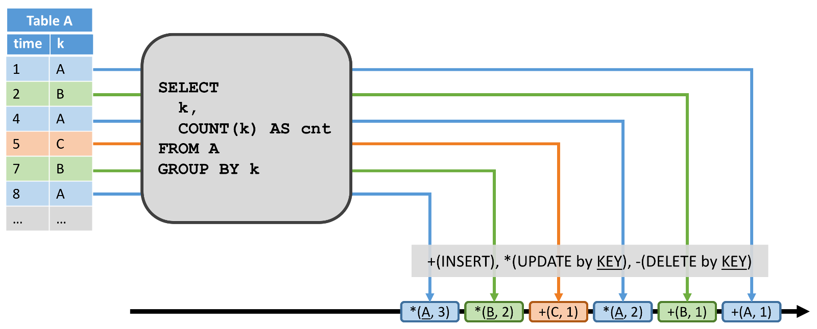
The row (1, A) which yields an insert into the dynamic table results in the +(A, 1) insert message. The row (4, A) which produces an update yields the *(A, 2) update message.

Common use cases for redo streams are to write the result of a query to an append-only storage system, like rolling files or a Kafka topic, or to a data store with keyed access, such as Cassandra, a relational DBMS, or a compacted Kafka topic. It is also possible to materialize a dynamic table as keyed state inside of the streaming application that evaluates the continuous query and make it queryable from external systems. With this design Flink itself maintains the result of a continuous SQL query on a stream and serves key lookups on the result table, for instance from a dashboard application.

What will Change When Switching to Dynamic Tables? #

In version 1.2, all streaming operators of Flink’s relational APIs, like filter, project, and group window aggregates, only emit new rows and are not capable of updating previously emitted results. In contrast, dynamic table are able to handle update and delete modifications. Now you might ask yourself, How does the processing model of the current version relate to the new dynamic table model? Will the semantics of the APIs completely change and do we need to reimplement the APIs from scratch to achieve the desired semantics?

The answer to all these questions is simple. The current processing model is a subset of the dynamic table model. Using the terminology we introduced in this post, the current model converts a stream into a dynamic table in append mode, i.e., an infinitely growing table. Since all operators only accept insert changes and produce insert changes on their result table (i.e., emit new rows), all supported queries result in dynamic append tables, which are converted back into DataStreams using the redo model for append-only tables. Consequently, the semantics of the current model are completely covered and preserved by the new dynamic table model.

Conclusion and Outlook #

Flink’s relational APIs are great to implement stream analytics applications in no time and used in several production settings. In this blog post we discussed the future of the Table API and SQL. This effort will make Flink and stream processing accessible to more people. Moreover, the unified semantics for querying historic and real-time data as well as the concept of querying and maintaining dynamic tables will enable and significantly ease the implementation of many exciting use cases and applications. As this post was focusing on the semantics of relational queries on streams and dynamic tables, we did not discuss the details of how a query will be executed, which includes the internal implementation of retractions, handling of late events, support for early results, and bounding space requirements. We plan to publish a follow up blog post on this topic at a later point in time.

In recent months, many members of the Flink community have been discussing and contributing to the relational APIs. We made great progress so far. While most work has focused on processing streams in append mode, the next steps on the agenda are to work on dynamic tables to support queries that update their results. If you are excited about the idea of processing streams with SQL and would like to contribute to this effort, please give feedback, join the discussions on the mailing list, or grab a JIRA issue to work on.