Flink SQL Demo: Building an End-to-End Streaming Application

Apache Flink 1.11 has released many exciting new features, including many developments in Flink SQL which is evolving at a fast pace. This article takes a closer look at how to quickly build streaming applications with Flink SQL from a practical point of view.

In the following sections, we describe how to integrate Kafka, MySQL, Elasticsearch, and Kibana with Flink SQL to analyze e-commerce user behavior in real-time. All exercises in this blogpost are performed in the Flink SQL CLI, and the entire process uses standard SQL syntax, without a single line of Java/Scala code or IDE installation. The final result of this demo is shown in the following figure:

Preparation #

Prepare a Linux or MacOS computer with Docker installed.

Starting the Demo Environment #

The components required in this demo are all managed in containers, so we will use docker-compose to start them. First, download the docker-compose.yml file that defines the demo environment, for example by running the following commands:

mkdir flink-sql-demo; cd flink-sql-demo;
wget https://raw.githubusercontent.com/wuchong/flink-sql-demo/v1.11-EN/docker-compose.yml

The Docker Compose environment consists of the following containers:

• Flink SQL CLI: used to submit queries and visualize their results.
• Flink Cluster: a Flink JobManager and a Flink TaskManager container to execute queries.
• MySQL: MySQL 5.7 and a pre-populated category table in the database. The category table will be joined with data in Kafka to enrich the real-time data.
• Kafka: mainly used as a data source. The DataGen component automatically writes data into a Kafka topic.
• Zookeeper: this component is required by Kafka.
• Elasticsearch: mainly used as a data sink.
• Kibana: used to visualize the data in Elasticsearch.
• DataGen: the data generator. After the container is started, user behavior data is automatically generated and sent to the Kafka topic. By default, 2000 data entries are generated each second for about 1.5 hours. You can modify DataGen’s speedup parameter in docker-compose.yml to adjust the generation rate (which takes effect after Docker Compose is restarted).

To start all containers, run the following command in the directory that contains the docker-compose.yml file.

docker-compose up -d

This command automatically starts all the containers defined in the Docker Compose configuration in a detached mode. Run docker ps to check whether the 9 containers are running properly. You can also visit http://localhost:5601/ to see if Kibana is running normally.

Don’t forget to run the following command to stop all containers after you finished the tutorial:

docker-compose down

Entering the Flink SQL CLI client #

To enter the SQL CLI client run:

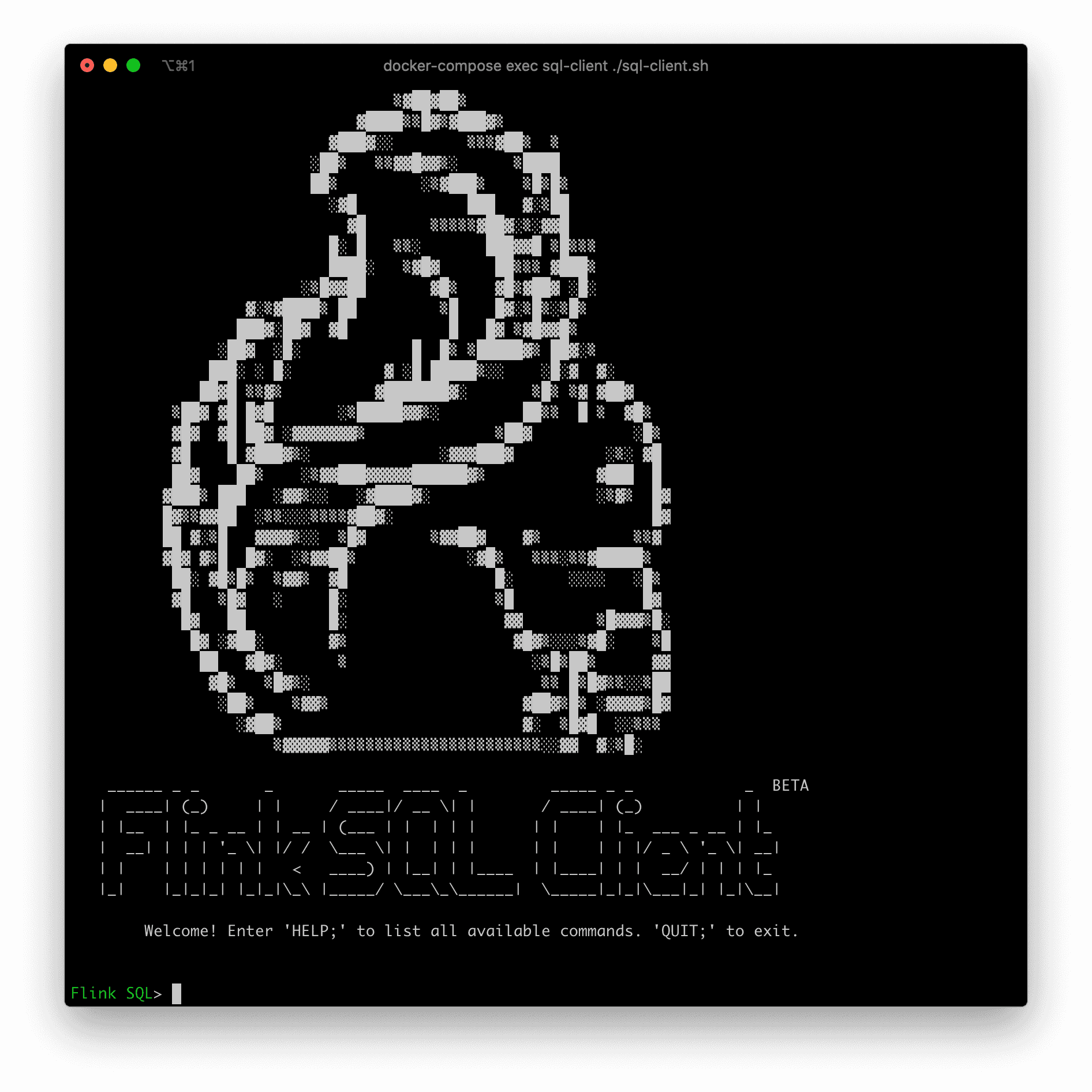
docker-compose exec sql-client ./sql-client.sh

The command starts the SQL CLI client in the container. You should see the welcome screen of the CLI client.

Creating a Kafka table using DDL #

The DataGen container continuously writes events into the Kafka user_behavior topic. This data contains the user behavior on the day of November 27, 2017 (behaviors include “click”, “like”, “purchase” and “add to shopping cart” events). Each row represents a user behavior event, with the user ID, product ID, product category ID, event type, and timestamp in JSON format. Note that the dataset is from the Alibaba Cloud Tianchi public dataset.

In the directory that contains docker-compose.yml, run the following command to view the first 10 data entries generated in the Kafka topic:

docker-compose exec kafka bash -c 'kafka-console-consumer.sh --topic user_behavior --bootstrap-server kafka:9094 --from-beginning --max-messages 10'

{"user_id": "952483", "item_id":"310884", "category_id": "4580532", "behavior": "pv", "ts": "2017-11-27T00:00:00Z"}
{"user_id": "794777", "item_id":"5119439", "category_id": "982926", "behavior": "pv", "ts": "2017-11-27T00:00:00Z"}
...

In order to make the events in the Kafka topic accessible to Flink SQL, we run the following DDL statement in SQL CLI to create a table that connects to the topic in the Kafka cluster:

CREATE TABLE user_behavior (
    user_id BIGINT,
    item_id BIGINT,
    category_id BIGINT,
    behavior STRING,
    ts TIMESTAMP(3),
    proctime AS PROCTIME(),   -- generates processing-time attribute using computed column
    WATERMARK FOR ts AS ts - INTERVAL '5' SECOND  -- defines watermark on ts column, marks ts as event-time attribute
) WITH (
    'connector' = 'kafka',  -- using kafka connector
    'topic' = 'user_behavior',  -- kafka topic
    'scan.startup.mode' = 'earliest-offset',  -- reading from the beginning
    'properties.bootstrap.servers' = 'kafka:9094',  -- kafka broker address
    'format' = 'json'  -- the data format is json
);

The above snippet declares five fields based on the data format. In addition, it uses the computed column syntax and built-in PROCTIME() function to declare a virtual column that generates the processing-time attribute. It also uses the WATERMARK syntax to declare the watermark strategy on the ts field (tolerate 5-seconds out-of-order). Therefore, the ts field becomes an event-time attribute. For more information about time attributes and DDL syntax, see the following official documents:

• Time attributes in Flink’s Table API & SQL
• DDL Syntax in Flink SQL

After creating the user_behavior table in the SQL CLI, run SHOW TABLES; and DESCRIBE user_behavior; to see registered tables and table details. Also, run the command SELECT * FROM user_behavior; directly in the SQL CLI to preview the data (press q to exit).

Next, we discover more about Flink SQL through three real-world scenarios.

Hourly Trading Volume #

Creating an Elasticsearch table using DDL #

Let’s create an Elasticsearch result table in the SQL CLI. We need two columns in this case: hour_of_day and buy_cnt (trading volume).

CREATE TABLE buy_cnt_per_hour (
    hour_of_day BIGINT,
    buy_cnt BIGINT
) WITH (
    'connector' = 'elasticsearch-7', -- using elasticsearch connector
    'hosts' = 'http://elasticsearch:9200',  -- elasticsearch address
    'index' = 'buy_cnt_per_hour'  -- elasticsearch index name, similar to database table name
);

There is no need to create the buy_cnt_per_hour index in Elasticsearch in advance since Elasticsearch will automatically create the index if it does not exist.

Submitting a Query #

The hourly trading volume is the number of “buy” behaviors completed each hour. Therefore, we can use a TUMBLE window function to assign data into hourly windows. Then, we count the number of “buy” records in each window. To implement this, we can filter out the “buy” data first and then apply COUNT(*).

INSERT INTO buy_cnt_per_hour
SELECT HOUR(TUMBLE_START(ts, INTERVAL '1' HOUR)), COUNT(*)
FROM user_behavior
WHERE behavior = 'buy'
GROUP BY TUMBLE(ts, INTERVAL '1' HOUR);

Here, we use the built-in HOUR function to extract the value for each hour in the day from a TIMESTAMP column. Use INSERT INTO to start a Flink SQL job that continuously writes results into the Elasticsearch buy_cnt_per_hour index. The Elasticearch result table can be seen as a materialized view of the query. You can find more information about Flink’s window aggregation in the Apache Flink documentation.

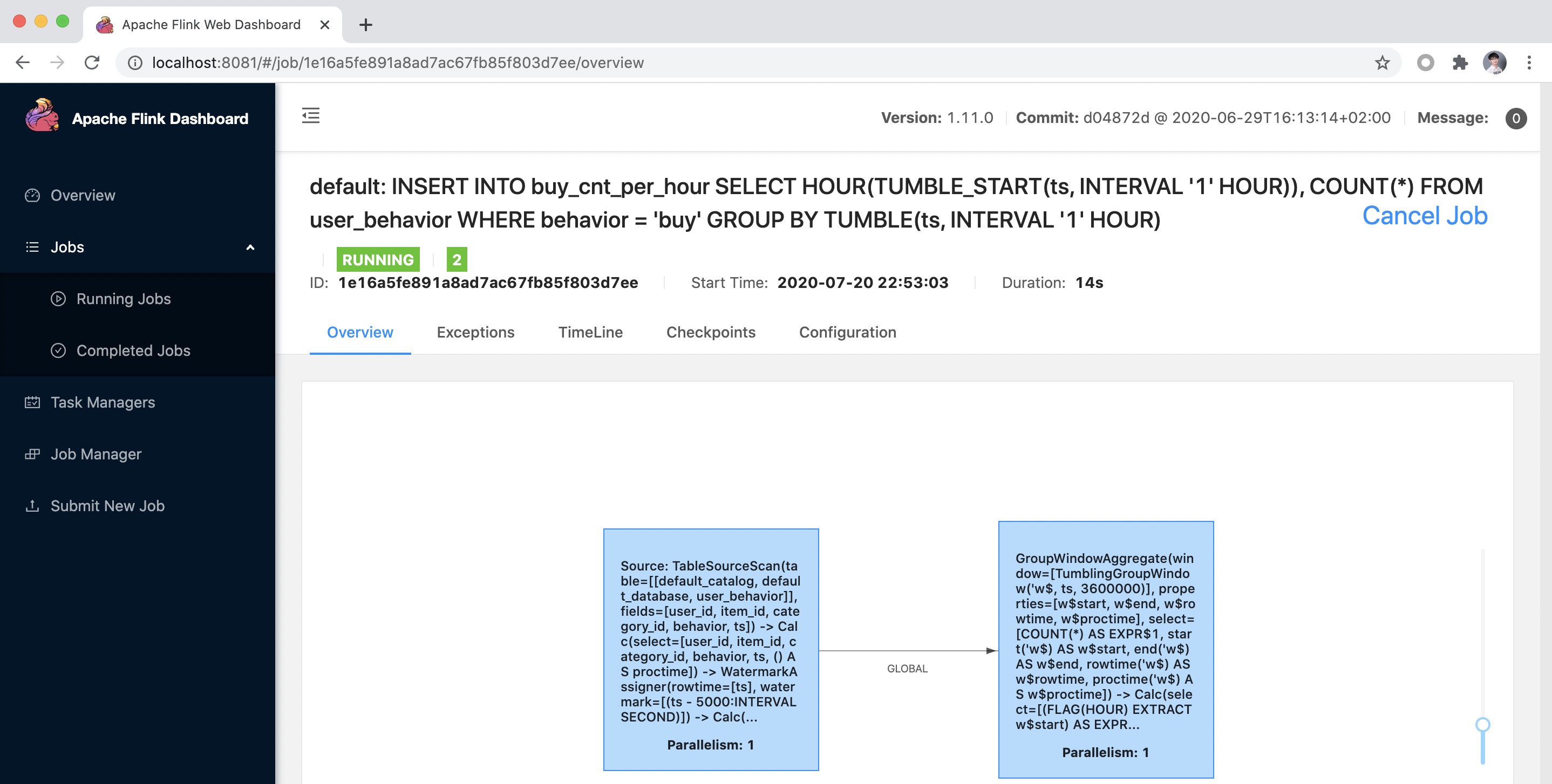
After running the previous query in the Flink SQL CLI, we can observe the submitted task on the Flink Web UI. This task is a streaming task and therefore runs continuously.

Using Kibana to Visualize Results #

Access Kibana at http://localhost:5601. First, configure an index pattern by clicking “Management” in the left-side toolbar and find “Index Patterns”. Next, click “Create Index Pattern” and enter the full index name buy_cnt_per_hour to create the index pattern. After creating the index pattern, we can explore data in Kibana.

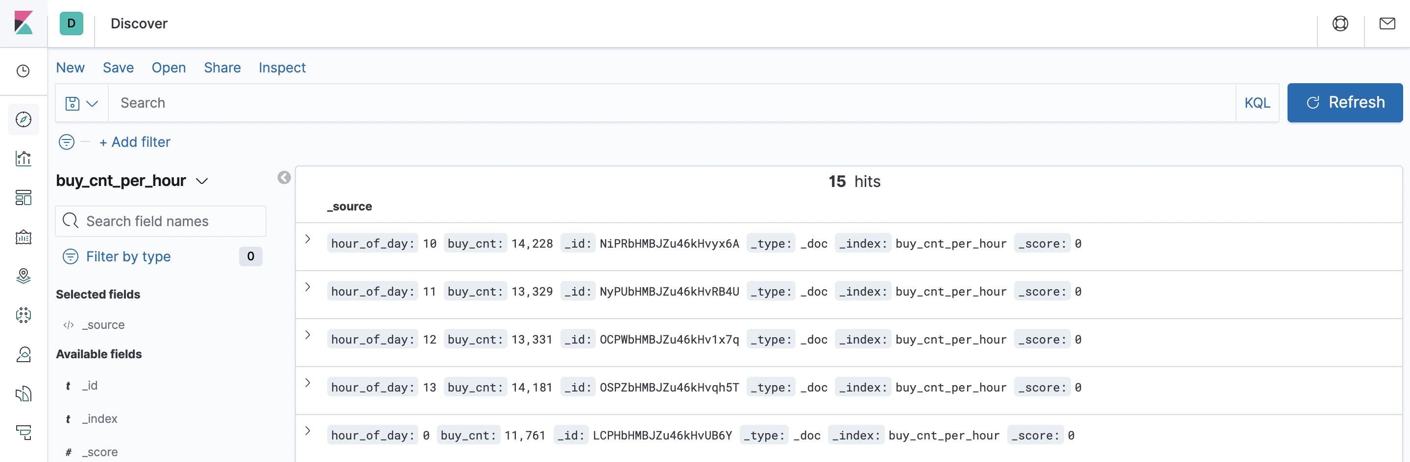
Click “Discover” in the left-side toolbar. Kibana lists the content of the created index.

Next, create a dashboard to display various views. Click “Dashboard” on the left side of the page to create a dashboard named “User Behavior Analysis”. Then, click “Create New” to create a new view. Select “Area” (area graph), then select the buy_cnt_per_hour index, and draw the trading volume area chart as illustrated in the configuration on the left side of the following diagram. Apply the changes by clicking the “▶” play button. Then, save it as “Hourly Trading Volume”.

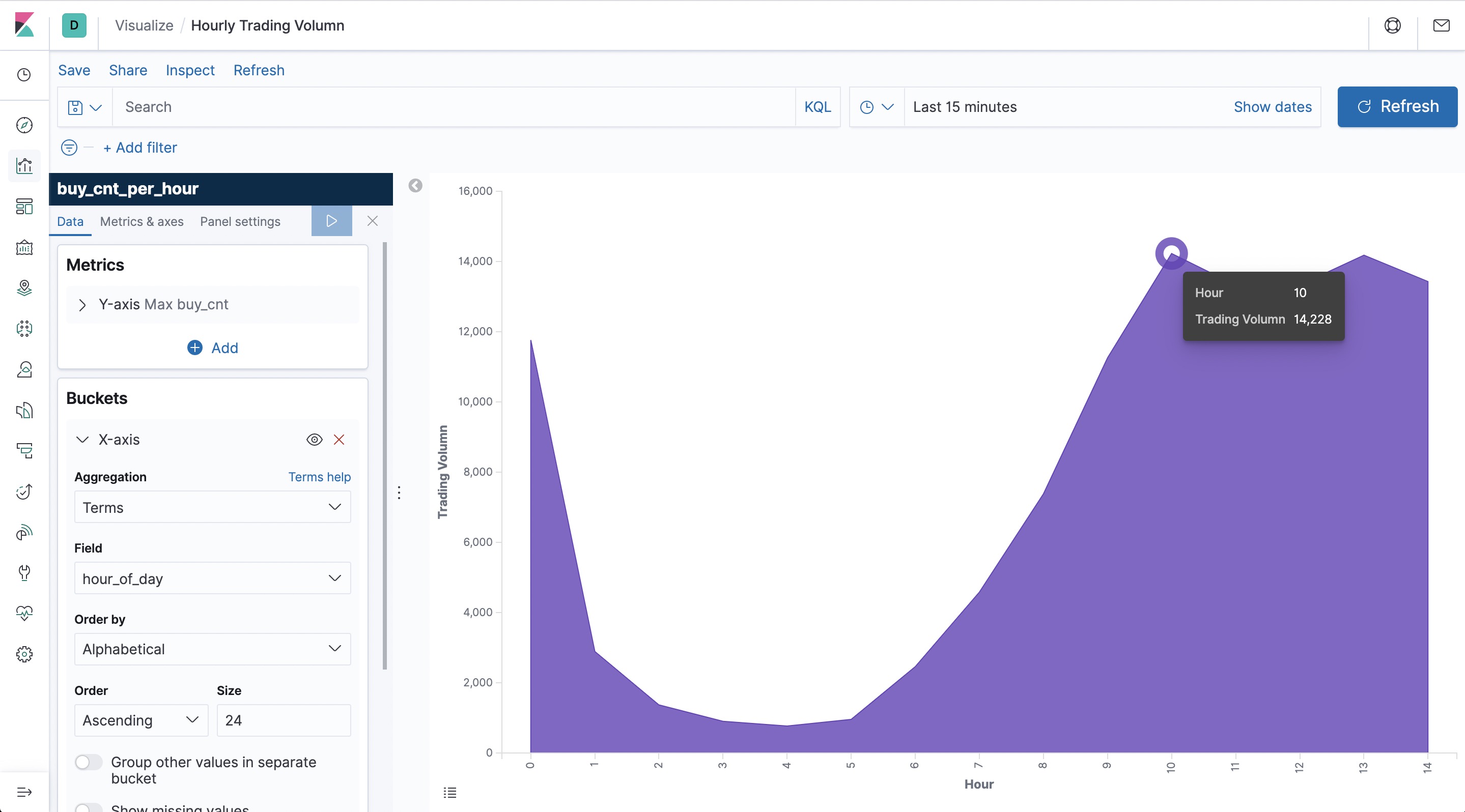
You can see that during the early morning hours the number of transactions have the lowest value for the entire day.

As real-time data is added into the indices, you can enable auto-refresh in Kibana to see real-time visualization changes and updates. You can do so by clicking the time picker and entering a refresh interval (e.g. 3 seconds) in the “Refresh every” field.

Cumulative number of Unique Visitors every 10-min #

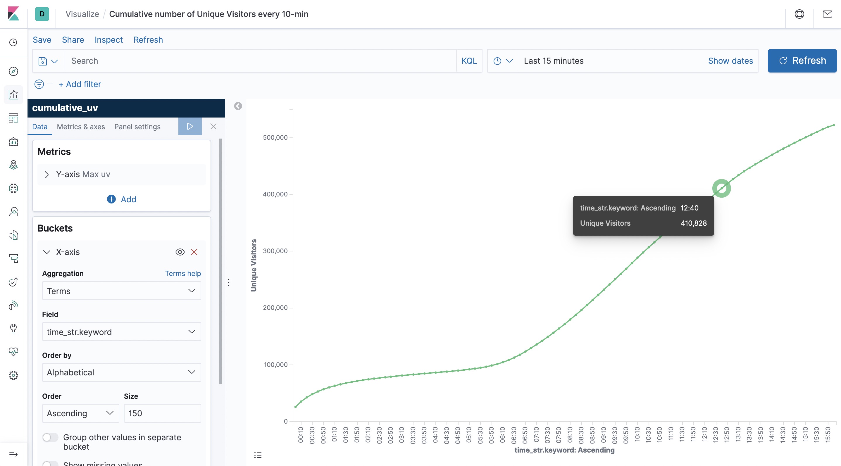
Another interesting visualization is the cumulative number of unique visitors (UV). For example, the number of UV at 10:00 represents the total number of UV from 00:00 to 10:00. Therefore, the curve is monotonically increasing.

Let’s create another Elasticsearch table in the SQL CLI to store the UV results. This table contains 3 columns: date, time and cumulative UVs. The date_str and time_str column are defined as primary key, Elasticsearch sink will use them to calculate the document ID and work in upsert mode to update UV values under the document ID.

CREATE TABLE cumulative_uv (
    date_str STRING,
    time_str STRING,
    uv BIGINT,
    PRIMARY KEY (date_str, time_str) NOT ENFORCED
) WITH (
    'connector' = 'elasticsearch-7',
    'hosts' = 'http://elasticsearch:9200',
    'index' = 'cumulative_uv'
);

We can extract the date and time using DATE_FORMAT function based on the ts field. As the section title describes, we only need to report every 10 minutes. So, we can use SUBSTR and the string concat function || to convert the time value into a 10-minute interval time string, such as 12:00, 12:10. Next, we group data by date_str and perform a COUNT DISTINCT aggregation on user_id to get the current cumulative UV in this day. Additionally, we perform a MAX aggregation on time_str field to get the current stream time: the maximum event time observed so far. As the maximum time is also a part of the primary key of the sink, the final result is that we will insert a new point into the elasticsearch every 10 minute. And every latest point will be updated continuously until the next 10-minute point is generated.

INSERT INTO cumulative_uv
SELECT date_str, MAX(time_str), COUNT(DISTINCT user_id) as uv
FROM (
  SELECT
    DATE_FORMAT(ts, 'yyyy-MM-dd') as date_str,
    SUBSTR(DATE_FORMAT(ts, 'HH:mm'),1,4) || '0' as time_str,
    user_id
  FROM user_behavior)
GROUP BY date_str;

After submitting this query, we create a cumulative_uv index pattern in Kibana. We then create a “Line” (line graph) on the dashboard, by selecting the cumulative_uv index, and drawing the cumulative UV curve according to the configuration on the left side of the following figure before finally saving the curve.

Top Categories #

The last visualization represents the category rankings to inform us on the most popular categories in our e-commerce site. Since our data source offers events for more than 5,000 categories without providing any additional significance to our analytics, we would like to reduce it so that it only includes the top-level categories. We will use the data in our MySQL database by joining it as a dimension table with our Kafka events to map sub-categories to top-level categories.

Create a table in the SQL CLI to make the data in MySQL accessible to Flink SQL.

CREATE TABLE category_dim (
    sub_category_id BIGINT,
    parent_category_name STRING
) WITH (
    'connector' = 'jdbc',
    'url' = 'jdbc:mysql://mysql:3306/flink',
    'table-name' = 'category',
    'username' = 'root',
    'password' = '123456',
    'lookup.cache.max-rows' = '5000',
    'lookup.cache.ttl' = '10min'
);

The underlying JDBC connector implements the LookupTableSource interface, so the created JDBC table category_dim can be used as a temporal table (i.e. lookup table) out-of-the-box in the data enrichment.

In addition, create an Elasticsearch table to store the category statistics.

CREATE TABLE top_category (
    category_name STRING PRIMARY KEY NOT ENFORCED,
    buy_cnt BIGINT
) WITH (
    'connector' = 'elasticsearch-7',
    'hosts' = 'http://elasticsearch:9200',
    'index' = 'top_category'
);

In order to enrich the category names, we use Flink SQL’s temporal table joins to join a dimension table. You can access more information about temporal joins in the Flink documentation.

Additionally, we use the CREATE VIEW syntax to register the query as a logical view, allowing us to easily reference this query in subsequent queries and simplify nested queries. Please note that creating a logical view does not trigger the execution of the job and the view results are not persisted. Therefore, this statement is lightweight and does not have additional overhead.

CREATE VIEW rich_user_behavior AS
SELECT U.user_id, U.item_id, U.behavior, C.parent_category_name as category_name
FROM user_behavior AS U LEFT JOIN category_dim FOR SYSTEM_TIME AS OF U.proctime AS C
ON U.category_id = C.sub_category_id;

Finally, we group the dimensional table by category name to count the number of buy events and write the result to Elasticsearch’s top_category index.

INSERT INTO top_category
SELECT category_name, COUNT(*) buy_cnt
FROM rich_user_behavior
WHERE behavior = 'buy'
GROUP BY category_name;

After submitting the query, we create a top_category index pattern in Kibana. We then create a “Horizontal Bar” (bar graph) on the dashboard, by selecting the top_category index and drawing the category ranking according to the configuration on the left side of the following diagram before finally saving the list.

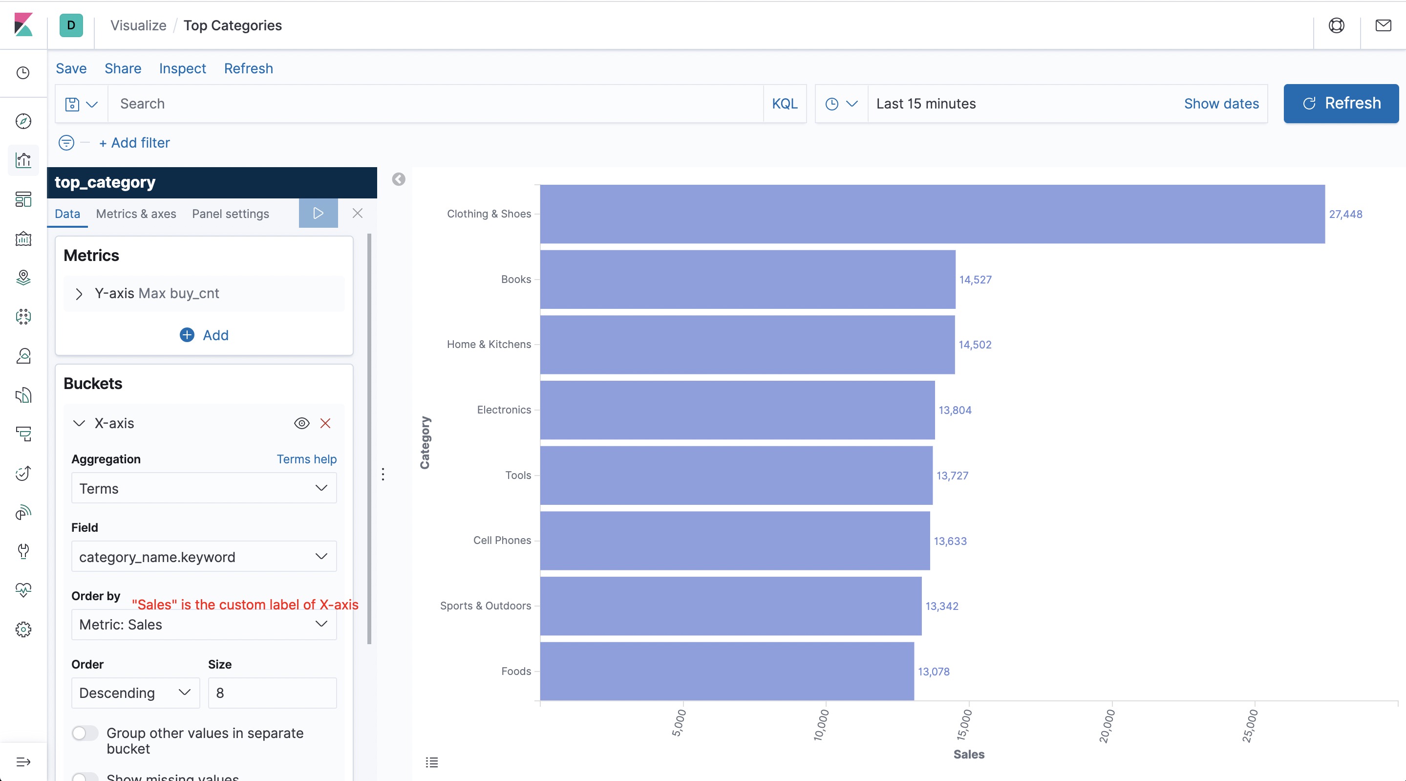
As illustrated in the diagram, the categories of clothing and shoes exceed by far other categories on the e-commerce website.

We have now implemented three practical applications and created charts for them. We can now return to the dashboard page and drag-and-drop each view to give our dashboard a more formal and intuitive style, as illustrated in the beginning of the blogpost. Of course, Kibana also provides a rich set of graphics and visualization features, and the user_behavior logs contain a lot more interesting information to explore. Using Flink SQL, you can analyze data in more dimensions, while using Kibana allows you to display more views and observe real-time changes in its charts!

Summary #

In the previous sections, we described how to use Flink SQL to integrate Kafka, MySQL, Elasticsearch, and Kibana to quickly build a real-time analytics application. The entire process can be completed using standard SQL syntax, without a line of Java or Scala code. We hope that this article provides some clear and practical examples of the convenience and power of Flink SQL, featuring an easy connection to various external systems, native support for event time and out-of-order handling, dimension table joins and a wide range of built-in functions. We hope you have fun following the examples in this blogpost!