Exploring fine-grained recovery of bounded data sets on Flink

Apache Flink is a very versatile tool for all kinds of data processing workloads. It can process incoming data within a few milliseconds or crunch through petabytes of bounded datasets (also known as batch processing).

Processing efficiency is not the only parameter users of data processing systems care about. In the real world, system outages due to hardware or software failure are expected to happen all the time. For unbounded (or streaming) workloads, Flink is using periodic checkpoints to allow for reliable and correct recovery. In case of bounded data sets, having a reliable recovery mechanism is mission critical — as users do not want to potentially lose many hours of intermediate processing results.

Apache Flink 1.9 introduced fine-grained recovery into its internal workload scheduler. The Flink APIs that are made for bounded workloads benefit from this change by individually recovering failed operators, re-using results from the previous processing step.

In this blog post, we are going to give an overview over these changes, and we will experimentally validate their effectiveness.

How does fine-grained recovery work? #

For streaming jobs (and in pipelined mode for batch jobs), Flink is using a coarse-grained restart-strategy: upon failure, the entire job is restarted (but streaming jobs have an entirely different fault-tolerance model, using checkpointing)

For batch jobs, we can use a more sophisticated recovery strategy, by using cached intermediate results, thus only restarting parts of the pipeline.

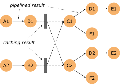
Let’s look at the topology below: Some connections are pipelined (between A1 and B1, as well as A2 and B2) – data is immediately streamed from operator A1 to B1.

However the output of B1 and B2 is cached on disk (indicated by the grey box). We call such connections blocking. If there’s a failure in the steps succeeding B1 and B2 and the results of B1 and B2 have already been produced, we don’t need to reprocess this part of the pipeline – we can reuse the cached result.

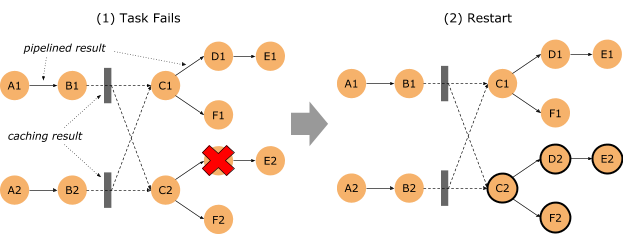
Looking at the case of a failure (here of D2), we see that we do not need to restart the entire job. Restarting C2 and all dependent tasks is sufficient. This is possible because we can read the cached results of B1 and B2. We call this recovery mechanism “fine-grained”, as we only restart parts of the topology to recover from a failure – reducing the recovery time, resource consumption and overall job runtime.

Experimenting with fine-grained recovery #

To validate the implementation, we’ve conducted a small experiment. The following sections will describe the setup, the experiment and the results.

Setup #

Hardware: The experiment was performed on an idle MacBook Pro 2016 (16 GB of memory, SSD storage).

Test Job: We used a modified version (for instrumentation only) of the TPC-H Query 3 example that is part of the Flink batch (DataSet API) examples, running on Flink 1.12

This is the topology of the query:

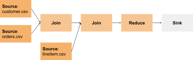
It has many blocking data exchanges where we cache intermediate results, if executed in batch mode.

Test Data: We generated a TPC-H dataset of 150 GB as the input.

Cluster: We were running 4 TaskManagers with 2 slots each and 1 JobManager in standalone mode.

Running this test job takes roughly 15 minutes with the given hardware and data.

For inducing failures into the job, we decided to randomly throw exceptions in the operators. This has a number of benefits compared to randomly killing entire TaskManagers:

• Killing a TaskManager would require starting and registering a new TaskManager — which introduces an uncontrollable factor into our benchmark: We don’t want to test how quickly Flink is reconciling a cluster.
• Killing an entire TaskManager would bring down on average 1/4th of all running operators. In larger production setups, a failure usually affects only a smaller fraction of all running operators. The differences between the execution modes would be less obvious if we killed entire TaskManagers.
• Keeping TaskManagers across failures helps to better simulate using an external shuffle service, as intermediate results are preserved despite a failure.

The failures are controlled by a central “failure coordinator” which decides when to kill which operator.

Failures are artificially triggered based on a configured mean failure frequency. The failures follow an exponential distribution, which is suitable for simulating continuous and independent failures at a configured average rate.

The Experiment #

We were running the job with two parameters which we varied in the benchmark:

• Execution Mode: BATCH or PIPELINED.

  In PIPELINED mode, except for data exchanges susceptible for deadlocks all exchanges are pipelined (e.g. upstream operators are streaming their result downstream). A failure means that we have to restart the entire job, and start the processing from scratch.

  In BATCH mode, all shuffles and broadcasts are persisted before downstream consumption. You can imagine the execution to happen in steps. Since we are persisting intermediate results in BATCH mode, we do not have to reprocess all upstream operators in case of an (induced) failure. We just have to restart the step that was in progress during the failure.

• Mean Failure Frequency: This parameter controls the frequency of failures induced into the running job. If the parameter is set to 5 minutes, on average, a failure occurs every 5 minutes. The failures are following an exponential distribution. We’ve chosen values between 15 minutes and 20 seconds.

Each configuration combination was executed at least 3 times. We report the average execution time. This is necessary due to the probabilistic behavior of the induced failures.

The Results #

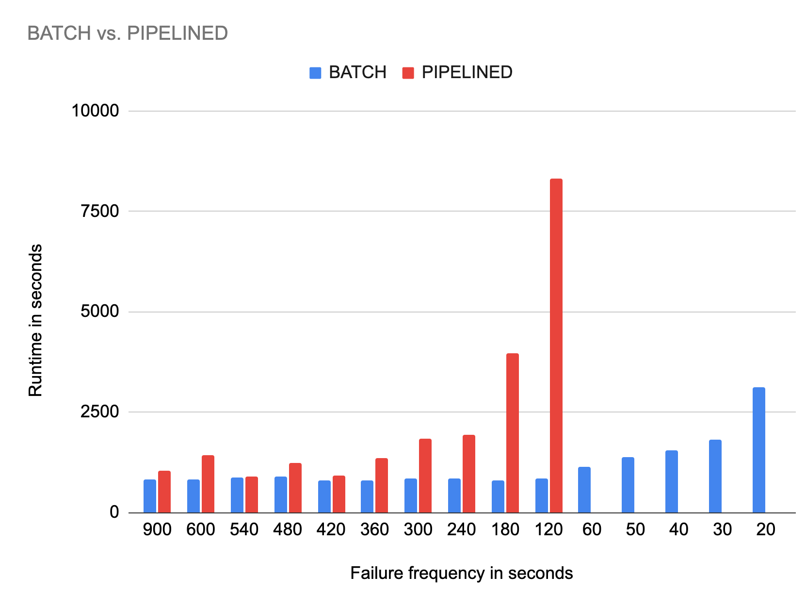
The chart below shows the execution time in seconds for each batch and pipelined execution with different failure frequencies.

We will now discuss some findings:

1. Execution time with rare failures: Looking at the first few results on the left, where we compare the behavior with a mean failure frequency of 15 (=900s), 10 (=600s), 9 (=540s), 8 (=480s), 7 (=420s) minutes. The execution times are mostly the same, around 15 minutes. The batch execution time is usually lower, and more predictable. This behavior is easy to explain. If an error occurred later in the execution, the pipelined mode needs to start from scratch, while the batch mode can re-use previous intermediate results. The variances in runtime can be explained by statistical effects: if an error happens to be induced close to the end of a pipelined mode run, the entire job needs to rerun.
2. Execution time with frequent failures: The results “in the middle”, with failure frequencies of 6, 5, 4, 3 and 2 minutes show that the pipelined mode execution gets unfeasible at some point: If failures happen on average every 3 minutes, the average execution time reaches more than 60 minutes, for failures every 2 minutes the time spikes to more than 120 minutes. The pipelined job is unable to finish the execution, only if we happen to find a window where no failure is induced for 15 minutes, the pipelined job manages to produce the final result. For more frequent failures, the pipelined mode did not manage to finish at all.
3. How many failures can the batch mode sustain? The last numbers, with failure frequencies between 60 and 20 seconds are probably a bit unrealistic for real world scenarios. But we wanted to investigate how frequent failures can become for the batch mode to become unfeasible. With failures induced every 30 seconds, the average execution time is 30 minutes. In other words, even if you have two failures per minute, your execution time only doubles in this case. The batch mode is much more predictable and well behaved when it comes to execution times.

Conclusion #

Based on these results, it makes a lot of sense to use the batch execution mode for batch workloads, as the resource consumption and overall execution times are substantially lower compared to the pipelined execution mode.

In general, we recommend conducting your own performance experiments on your own hardware and with your own workloads, as results might vary from what we’ve presented here. Despite the findings here, the pipelined mode probably has some performance advantages in environments with rare failures and slower I/O (for example when using spinning disks, or network attached disks). On the other hand, CPU intensive workloads might benefit from the batch mode even in slow I/O environments.

We should also note that the caching (and subsequent reprocessing on failure) only works if the cached results are still present – this is currently only the case, if the TaskManager survives a failure. However, this is an unrealistic assumption as many failures would cause the TaskManager process to die. To mitigate this limitation, data processing frameworks employ external shuffle services that persist the cached results independent of the data processing framework. Since Flink 1.9, there is support for a pluggable shuffle service, and there are tickets for adding implementations for YARN (FLINK-13247) and Kubernetes (FLINK-13246). Once these implementations are added, TaskManagers can recover cached results even if the process or machine got killed.

Despite these considerations, we believe that fine-grained recovery is a great improvement for Flink’s batch capabilities, as it makes the framework much more efficient, even in unstable environments.