A Rundown of Batch Execution Mode in the DataStream API

March 11, 2021 - Dawid Wysakowicz (@dwysakowicz)

Flink has been following the mantra that Batch is a Special Case of Streaming since the very early days. As the project evolved to address specific uses cases, different core APIs ended up being implemented for batch (DataSet API) and streaming execution (DataStream API), but the higher-level Table API/SQL was subsequently designed following this mantra of unification. With Flink 1.12, the community worked on bringing a similarly unified behaviour to the DataStream API, and took the first steps towards enabling efficient batch execution in the DataStream API.

The idea behind making the DataStream API a unified abstraction for batch and streaming execution instead of maintaining separate APIs is two-fold:

Reusability: efficient batch and stream processing under the same API would allow you to easily switch between both execution modes without rewriting any code. So, a job could be easily reused to process real-time and historical data.
Operational simplicity: providing a unified API would mean using a single set of connectors, maintaining a single codebase and being able to easily implement mixed execution pipelines e.g. for use cases like backfilling.

The difference between BATCH and STREAMING vs BOUNDED and UNBOUNDED is subtle, and a common source of confusion — so, let’s start by clarifying that. These terms might seem mostly interchangeable, but in reality serve different purposes:

Bounded and unbounded refer to the characteristics of the streams you want to process: whether or not they are known to have an end. The terms are also sometimes applied to the applications processing these streams: an application that only processes bounded streams is a bounded stream processing application that eventually finishes; while an unbounded stream processing application processes an unbounded stream and runs forever (or until canceled).

Batch and streaming are execution modes. Batch execution is only applicable to bounded streams/applications because it exploits the fact that it can process the whole data (e.g. from a partition) in a batch rather than event-by-event, and possibly execute different batches one after the other. Continuous streaming execution runs everything at the same time, continuously processes (small groups of) events and is applicable to both bounded and unbounded applications.

Based on that differentiation, there are two main scenarios that result of the combination of these properties:

A bounded Stream Processing Application that is executed in a batch mode, which you can call a Batch (Processing) Application.
An unbounded Stream Processing Application that is executed in a streaming mode. This is the combination that has been the primary use case for the DataStream API in Flink.

It’s also possible to have a bounded Stream Processing Application that is executed in streaming mode, but this combination is less significant and likely to be used e.g. in a test environment or in other rare corner cases.

Which API and execution mode should I use? #

Before going into the choice of execution mode, try looking at your use case from a different angle: do you need to process structured data? Does your data have a schema of some sort? The Table API/SQL will most likely be the right choice. In fact, the majority of batch use cases should be expressed with the Table API/SQL! Finite, bounded data can most often be organized, described with a schema and put into a catalog. This is where the SQL API shines, giving you a rich set of functions and operators out-of-the box with low-level optimizations and broad connector support, all supported by standard SQL. And it works for streaming use cases, as well!

However, if you need explicit control over the execution graph, you want to manually control the state of your operations, or you need to be able to upgrade Flink (which applies to unbounded applications), the DataStream API is the right choice. If the DataStream API sounds like the best fit for your use cases, the next decision is what execution mode to run your program in.

When should you use the batch mode, then?

The simple answer is if you run your computation on bounded, historic data. The batch mode has a few benefits:

In bounded data there is no such thing as late data. You do not need to think how to adjust the watermarking logic that you use in your application. In a streaming case, you need to maintain the order in which the records were written - which is often not possible to recreate when reading from e.g. historic files. In batch mode you don’t need to care about that as the data will be sorted according to the timestamp and “perfect” watermarks will be injected automatically.
The way streaming applications are scheduled and react upon failure have significant performance implications that can be optimized when dealing with bounded data. We recommend reading through the blogposts on pipelined region scheduling and fine-grained fault tolerance to better understand these performance implications.
It can simplify the operational overhead of setting up and maintaining your pipelines. For example, there is no need to configure checkpointing, which otherwise requires things like choosing a state backend or setting up distributed storage for checkpoints.

How to use the batch execution #

Once you have a good understanding of which execution mode is better suited to your use case, you can configure it via the execution.runtime-mode setting. There are three possible values:

STREAMING: The classic DataStream execution mode (default)
BATCH: Batch-style execution on the DataStream API
AUTOMATIC: Let the system decide based on the boundedness of the sources

This can be configured via command line parameters of bin/flink run ... when submitting a job:

$ bin/flink run -Dexecution.runtime-mode=BATCH examples/streaming/WordCount.jar

, or programmatically when creating/configuring the StreamExecutionEnvironment

StreamExecutionEnvironment env = StreamExecutionEnvironment.getExecutionEnvironment();
env.setRuntimeMode(RuntimeExecutionMode.BATCH);

We recommend passing the execution mode when submitting the job, in order to keep your code configuration-free and potentially be able to execute the same application in different execution modes.

Hello batch mode #

Now that you know how to set the execution mode, let’s try to write a simple word count program and see how it behaves depending on the chosen mode. The program is a variation of a standard word count, where we count number of orders placed in a given currency. We derive the number in 1-day windows. We read the input data from a new unified file source and then apply a window aggregation. Notice that we will be checking the side output for late arriving data, which can illustrate how watermarks behave differently in the two execution modes.

public class WindowWordCount {
	private static final OutputTag<String[]> LATE_DATA = new OutputTag<>(
		"late-data",
		BasicArrayTypeInfo.STRING_ARRAY_TYPE_INFO);

	public static void main(String[] args) throws Exception {

		StreamExecutionEnvironment env = StreamExecutionEnvironment.getExecutionEnvironment();
		ParameterTool config = ParameterTool.fromArgs(args);

		Path path = new Path(config.get("path"));
		SingleOutputStreamOperator<Tuple4<String, Integer, String, String>> dataStream = env
			.fromSource(
				FileSource.forRecordStreamFormat(new TsvFormat(), path).build(),
				WatermarkStrategy.<String[]>forBoundedOutOfOrderness(Duration.ofDays(1))
					.withTimestampAssigner(new OrderTimestampAssigner()),
				"Text file"
			)
			.keyBy(value -> value[4]) // group by currency
			.window(TumblingEventTimeWindows.of(Time.days(1)))
			.sideOutputLateData(LATE_DATA)
			.aggregate(
				new CountFunction(), // count number of orders in a given currency
				new CombineWindow());

		int i = 0;
		DataStream<String[]> lateData = dataStream.getSideOutput(LATE_DATA);
		try (CloseableIterator<String[]> results = lateData.executeAndCollect()) {
			while (results.hasNext()) {
				String[] late = results.next();
				if (i < 100) {
					System.out.println(Arrays.toString(late));
				}
				i++;
			}
		}
		System.out.println("Number of late records: " + i);

		try (CloseableIterator<Tuple4<String, Integer, String, String>> results 
				= dataStream.executeAndCollect()) {
			while (results.hasNext()) {
				System.out.println(results.next());
			}
		}
	}
}

If we simply execute the above program with:

$ bin/flink run examples/streaming/WindowWordCount.jar

it will be executed in a streaming mode by default. Because of that, it will use the given watermarking strategy and produce windows based on it. In real-time scenarios, it might happen that records do not adhere to watermarks and some records might actually be considered late, so you’ll get results like:

...
[1431681, 130936, F, 135996.21, NOK, 2020-04-11 07:53:02.674, 2-HIGH, Clerk#000000922, 0, quests. slyly regular platelets cajole ironic deposits: blithely even depos]
[1431744, 143957, F, 36391.24, CHF, 2020-04-11 07:53:27.631, 2-HIGH, Clerk#000000406, 0, eans. blithely special instructions are quickly. q]
[1431812, 58096, F, 55292.05, CAD, 2020-04-11 07:54:16.956, 2-HIGH, Clerk#000000561, 0, , regular packages use. slyly even instr]
[1431844, 77335, O, 415443.20, CAD, 2020-04-11 07:54:40.967, 2-HIGH, Clerk#000000446, 0, unts across the courts wake after the accounts! ruthlessly]
[1431968, 122005, F, 44964.19, JPY, 2020-04-11 07:55:42.661, 1-URGENT, Clerk#000000001, 0, nal theodolites against the slyly special packages poach blithely special req]
[1432097, 26035, F, 42464.15, CAD, 2020-04-11 07:57:13.423, 5-LOW, Clerk#000000213, 0, l accounts hang blithely. carefully blithe dependencies ]
[1432193, 97537, F, 87856.63, NOK, 2020-04-11 07:58:06.862, 4-NOT SPECIFIED, Clerk#000000356, 0, furiously furiously brave foxes. bo]
[1432291, 112045, O, 114327.52, JPY, 2020-04-11 07:59:12.912, 1-URGENT, Clerk#000000732, 0, ding to the fluffily ironic requests haggle carefully alongsid]
Number of late records: 1514
(GBP,374,2020-03-31T00:00:00Z,2020-04-01T00:00:00Z)
(HKD,401,2020-03-31T00:00:00Z,2020-04-01T00:00:00Z)
(CNY,402,2020-03-31T00:00:00Z,2020-04-01T00:00:00Z)
(CAD,392,2020-03-31T00:00:00Z,2020-04-01T00:00:00Z)
(JPY,411,2020-03-31T00:00:00Z,2020-04-01T00:00:00Z)
(CHF,371,2020-03-31T00:00:00Z,2020-04-01T00:00:00Z)
(NOK,370,2020-03-31T00:00:00Z,2020-04-01T00:00:00Z)
(RUB,365,2020-03-31T00:00:00Z,2020-04-01T00:00:00Z)
...

However, if you execute the exact same code using the batch execution mode:

$ bin/flink run -Dexecution.runtime-mode=BATCH examples/streaming/WordCount.jar

you’ll see that there won’t be any late records.

Number of late records: 0
(GBP,374,2020-03-31T00:00:00Z,2020-04-01T00:00:00Z)
(HKD,401,2020-03-31T00:00:00Z,2020-04-01T00:00:00Z)
(CNY,402,2020-03-31T00:00:00Z,2020-04-01T00:00:00Z)
(CAD,392,2020-03-31T00:00:00Z,2020-04-01T00:00:00Z)
(JPY,411,2020-03-31T00:00:00Z,2020-04-01T00:00:00Z)
(CHF,371,2020-03-31T00:00:00Z,2020-04-01T00:00:00Z)
(NOK,370,2020-03-31T00:00:00Z,2020-04-01T00:00:00Z)
(RUB,365,2020-03-31T00:00:00Z,2020-04-01T00:00:00Z)

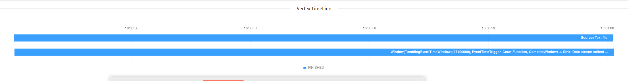
Also, if you compare the execution timelines of both runs, you’ll see that the jobs were scheduled differently. In the case of batch execution, the two stages were executed one after the other:

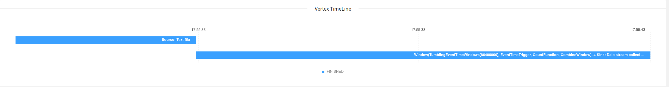
whereas for streaming both stages started at the same time.

Example: Two input operators #

Operators that process data from multiple inputs can be executed in both execution modes as well. Let’s see how we may implement a join of two data sets on a common key. (Disclaimer: Make sure to think first if you should use the Table API/SQL for your join!). We will enrich a stream of orders with information about the customer and we will make it run either of the two modes.

For this particular use case, the DataStream API provides a DataStream#join method that requires a window in which the join must happen; since we’ll process the data in bulk, we can use a GlobalWindow (that would otherwise not be very useful on its own in an unbounded case due to state size concerns):

DataStreamSource<String[]> orders = env
    .fromSource(
        FileSource.forRecordStreamFormat(new TsvFormat(), ordersPath).build(),
        WatermarkStrategy.<String[]>noWatermarks()
            .withTimestampAssigner((record, previous) -> -1),
        "Text file"
    );

Path customersPath = new Path(config.get("customers"));
DataStreamSource<String[]> customers = env
    .fromSource(
        FileSource.forRecordStreamFormat(new TsvFormat(), customersPath).build(),
        WatermarkStrategy.<String[]>noWatermarks()
            .withTimestampAssigner((record, previous) -> -1),
        "Text file"
    );

DataStream<Tuple2<String, String>> dataStream = orders.join(customers)
    .where(order -> order[1]).equalTo(customer -> customer[0]) // join on customer id
    .window(GlobalWindows.create())
    .trigger(ContinuousProcessingTimeTrigger.of(Time.seconds(5)))
    .apply(new ProjectFunction());

You might notice the ContinuousProcessingTimeTrigger. It is there for the application to produce results in a streaming mode. In a streaming application the GlobalWindow never finishes so we need to add a processing time trigger to emit results from time to time. We believe triggers are a way to control when to emit results, but are not part of the logic what to emit. Therefore we think it is safe to ignore those in case of batch mode and that’s what we do. In batch mode you will just get one final result for the join.

Looking into the future #

Support for efficient batch execution in the DataStream API was introduced in Flink 1.12 as a first step towards achieving a truly unified runtime for both batch and stream processing. This is not the end of the story yet! The community is still working on some optimizations and exploring more use cases that can be enabled with this new mode.

One of the first efforts we want to finalize is providing world-class support for transactional sinks in both execution modes, for bounded and unbounded streams. An experimental API for transactional sinks was already introduced in Flink 1.12, so we’re working on stabilizing it and would be happy to hear feedback about its current state!

We are also thinking how the two modes can be brought closer together and benefit from each other. A common pattern that we hear from users is bootstrapping state of a streaming job from a batch one. There are two somewhat different approaches we are considering here:

Having a mixed graph, where one of the branches would have only bounded sources and the other would reflect the unbounded part — you can think of such a graph as effectively two separate jobs. The bounded part would be executed first and sink into the state of a common vertex of the two parts. This jobs’ purpose would be to populate the state of the common operator. Once that job is done, we could proceed to running the unbounded part.
Another approach is to run the exact same program first on the bounded data. However, this time we wouldn’t assume completeness of the job; instead, we would produce the state of all operators up to a certain point in time and store it as a savepoint. Later on, we could use the savepoint to start the application on the unbounded data.

Lastly, to achieve feature parity with the DataSet API (Flink’s legacy API for batch-style execution), we are looking into the topic of iterations and how to meet the different usage patterns depending on the mode. In STREAMING mode, iterations serve as a loopback edge, but we don’t necessarily need to keep track of the iteration step. On the other hand, the iteration generation is vital for Machine Learning (ML) algorithms, which are the primary use case for iterations in BATCH mode.

Have you tried the new BATCH execution mode in the DataStream API? How was your experience? We are happy to hear your feedback and stories!