Getting into Low-Latency Gears with Apache Flink - Part Two

This series of blog posts present a collection of low-latency techniques in Flink. In part one, we discussed the types of latency in Flink and the way we measure end-to-end latency and presented a few techniques that optimize latency directly. In this post, we will continue with a few more direct latency optimization techniques. Just like in part one, for each optimization technique, we will clarify what it is, when to use it, and what to keep in mind when using it. We will also show experimental results to support our statements.

Direct latency optimization #

Spread work across time #

When you use timers or do windowing in a job, timer or window firing may create load spikes due to heavy computation or state access. If the allocated resources cannot cope with these load spikes, timer or window firing will take a long time to finish. This often results in high latency.

To avoid this situation, you should change your code to spread out the workload as much as possible such that you do not accumulate too much work to be done at a single point in time. In the case of windowing, you should consider using incremental window aggregation with AggregateFunction or ReduceFunction. In the case of timers in a ProcessFunction, the operations executed in the onTimer() method should be optimized such that the time spent there is reduced to a minimum. If you see latency spikes resulting from a global aggregation or if you need to collect events in a well-defined order to perform certain computations, you can consider adding a pre-aggregation phase in front of the current operator.

You can apply this optimization if you are using timer-based processing (e.g., timers, windowing) and an efficient aggregation can be applied whenever an event arrives instead of waiting for timers to fire.

Keep in mind that when you spread work across time, you should consider not only computation but also state access, especially when using RocksDB. Spreading one type of work while accumulating the other may result in higher latencies.

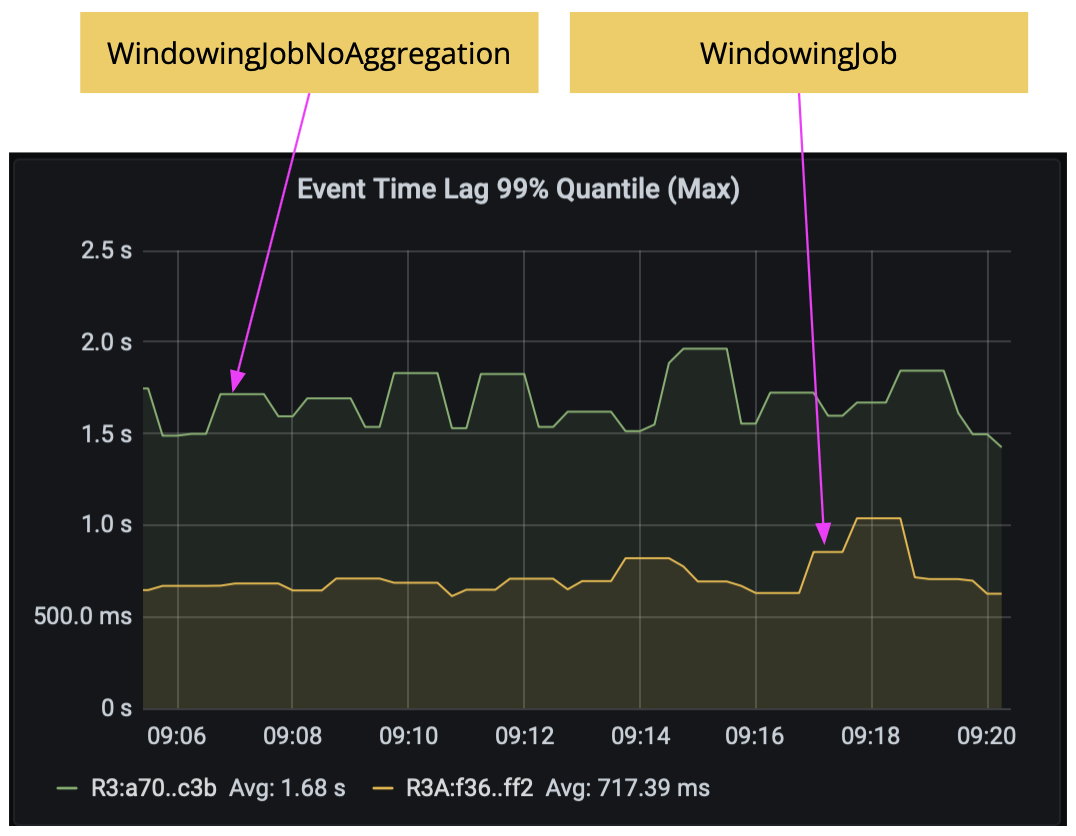
WindowingJob already does incremental window aggregation with AggregateFunction. To show the latency improvement of this technique, we compared WindowingJob with a variant that does not do incremental aggregation, WindowingJobNoAggregation, both running with the commonly used rocksdb state backend. As the results below show, without incremental window aggregation, the latency would increase from 720 ms to 1.7 seconds.

Access external systems efficiently #

Using async I/O #

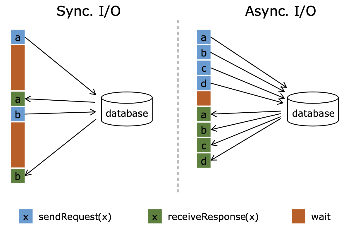
When interacting with external systems (e.g., RDBMS, object stores, web services) in a Flink job for data enrichment, the latency in getting responses from external systems often dominates the overall latency of the job. With Flink’s Async I/O API (e.g., AsyncDataStream.unorderedWait() or AsyncDataStream.orderedWait()), a single parallel function instance can handle many requests concurrently and receive responses asynchronously. This reduces latencies because the waiting time for responses is amortized over multiple requests.

You can apply this optimization if the client of your external system supports asynchronous requests. If it does not, you can use a thread pool of multiple clients to handle synchronous requests in parallel. You can also use a cache to speed up lookups if the data in the external system is not changing frequently. A cache, however, comes at the cost of working with outdated data.

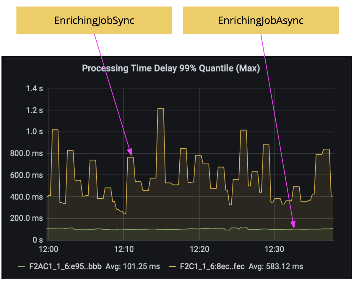
In this experiment, we simulated an external system that returns responses within 1 to 6 ms randomly, and we keep the external system response in a cache in our job for 1s. The results below show the comparison between two jobs: EnrichingJobSync and EnrichingJobAsync. By using async I/O, the latency was reduced from around 600 ms to 100 ms.

Using a streaming join #

If you are enriching a stream of events with an external database where the data changes frequently, and the changes can be converted to a data stream, then you have another option to use connected streams and a CoProcessFunction to do a streaming join. This can usually achieve lower latencies than the per-record lookups approach. An alternative approach is to pre-load external data into the job but a full streaming join can usually achieve better accuracy because it does not work with stale data and takes event-time into account. Please refer to this webinar for more details on streaming joins.

Tune checkpointing #

There are two aspects in checkpointing that impact latency: checkpoint alignment time as well as checkpoint frequency and duration in case of end-to-end exactly-once with transactional sinks.

Reduce checkpoint alignment time #

During checkpoint alignment, operators block the event processing from the channels where checkpoint barriers have been received in order to wait for the checkpoint barriers from other channels. Longer alignment time will result in higher latencies.

There are different ways to reduce checkpoint alignment time:

• Improve the throughput. Any improvement in throughput helps processing the buffers sitting in front of a checkpoint barrier faster.
• Scale up or scale out. This is the same as the technique of “allocate enough resources” described in part one. Increased processing power helps reducing backpressure and checkpoint alignment time.
• Use unaligned checkpointing. In this case, checkpoint barriers will not wait until the data is processed but skip over and pass on to the next operator immediately. Skipped-over data, however, has to be checkpointed as well in order to be consistent. Flink can also be configured to automatically switch over from aligned to unaligned checkpointing after a certain alignment time has passed.
• Buffer less data. You can reduce the buffered data size by tuning the number of exclusive and floating buffers. With less data buffered in the network stack, the checkpoint barrier can arrive at operators quicker. However, reducing buffers has an adverse effect on throughput and is just mentioned here for completeness. Flink 1.14 improves buffer handling by introducing a feature called buffer debloating. Buffer debloating can dynamically adjust buffer size based on the current throughput such that the buffered data can be worked off by the receiver within a configured fixed duration, e.g., 1 second. This reduces the buffered data during the alignment phase and can be used in combination with unaligned checkpointing to reduce the checkpoint alignment time.

Tune checkpoint duration and frequency #

If you are working with transactional sinks with exactly-once semantics, the output events are committed to external systems (e.g., Kafka) only upon checkpoint completion. In this case, tuning other options may not help if you do not tune checkpointing. Instead, you need to have fast and more frequent checkpointing.

To have fast checkpointing, you need to reduce the checkpoint duration. To achieve that, you can, for example, turn on rocksdb incremental checkpointing, reduce the state stored in Flink, clean up state that is not needed anymore, do not put cache into managed state, store only necessary fields in state, optimize the serialization format, etc. You can also scale up or scale out, same as the technique of “allocate enough resources” described in part one. This has two effects: it reduces backpressure because of the increased processing power, and with the increased parallelism, writing checkpoints to remote storage can finish quicker. You can also tune checkpoint alignment time, as described in the previous section, to reduce the checkpoint duration. If you use Flink 1.15 or later, you can enable the changelog feature. It may help to reduce the async duration of checkpointing.

To have more frequent checkpointing, you can reduce the checkpoint interval, the minimum pause between checkpoints, or use concurrent checkpoints. But keep in mind that concurrent checkpoints introduce more runtime overhead.

Another option is to not use exactly-once sinks but to switch to at-least-once sinks. The result of this is that you may have (correct but) duplicated output events, so this may require the downstream application that consumes the output events of your jobs to perform deduplication additionally.

Process events on arrival #

In a stream processing pipeline, there often exists a delay between the time an event is received and the time the event can be processed (e.g., after having seen all events up to a certain point in event time). The amount of delay may be significant for those pipelines with very low latency requirements. For example, a fraud detection job usually requires a sub-second level of latency. In this case, you could process events with ProcessFunction immediately when they arrive and deal with out-of-order events by yourself (in case of event-time processing) depending on your business requirements, e.g., drop or add them to the side output for special processing. Please refer to this Flink blog post for a great example of a low latency fraud detection job with implementation details.

You can apply this optimization if your job has a sub-second level latency requirement (e.g., hundreds of milliseconds) and the reduced watermarking interval still contributes a significant part of the latency.

Keep in mind that this may change your job logic considerably since you have to deal with out-of-order events by yourself.

Summary #

Following part one, this blog post presented a few more latency optimization techniques with a focus on direct latency optimization. In the next part, we will focus on techniques that optimize latency by increasing throughput. Stay tuned!